How to Use VLOOKUP in Excel or Google Sheets
VLOOKUP is more than a spreadsheet function; it's how you become a workplace hero. When you have two spreadsheets with different, but related sets of data like a list of customer addresses and a separate list of customer purchases, you can combine the data into one sheet. It's not hard to learn how to create a VLOOKUP formula, but most of your coworkers probably don't have this knowledge (and you don't have to tell them).
Over the years, I've used VLOOKUP to remain indispensible at all of my jobs in web publishing, because we often have a list of article URLs we want to track and then a giant CSV of all traffic data by page from Google Analytics. Here's how to use VLOOKUP in Microsoft Excel or Google Sheets. While the screenshots here are from Excel, the process works exactly the same way in Sheets.
1. Put both sheets into the same file, but in separate tabs. If you have the data you want to combine in separate files, create a new tab in one of them and copy over the data from the other.
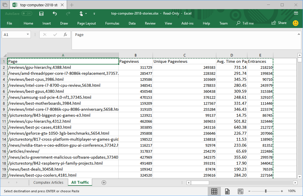
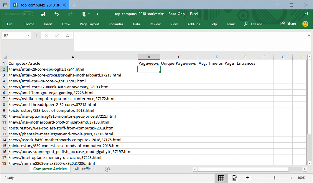
Article continues belowFor example, I started with a list of articles we wrote at Computex then downloaded a spreadsheet with traffic data from Google, which I moved over to a tab on the first sheet (numbers here are fake).
2. Navigate to the tab where you want to import the numbers and click into the first cell where you want them to appear. In my case, it was the tab with the list of Computex articles.
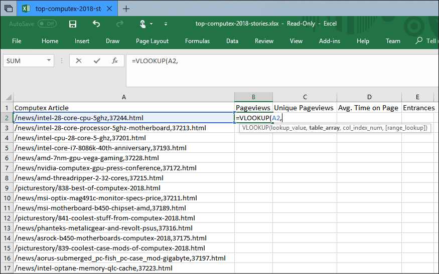
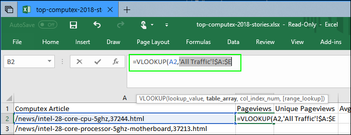
3. Type =VLOOKUP( then enter the cell number for the field you want to match followed by a comma. Since the article URL is the common field in my case, I'm selecting cell A2.
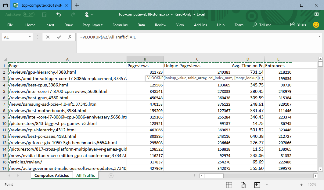
4. Select all the cells that contain data you want to import on the other tab. I recommend selecting the entire columns. Excel or Sheets will fill in the tab name and cell range (ex: 'All Traffic'!A:E).
Get Tom's Hardware's best news and in-depth reviews, straight to your inbox.
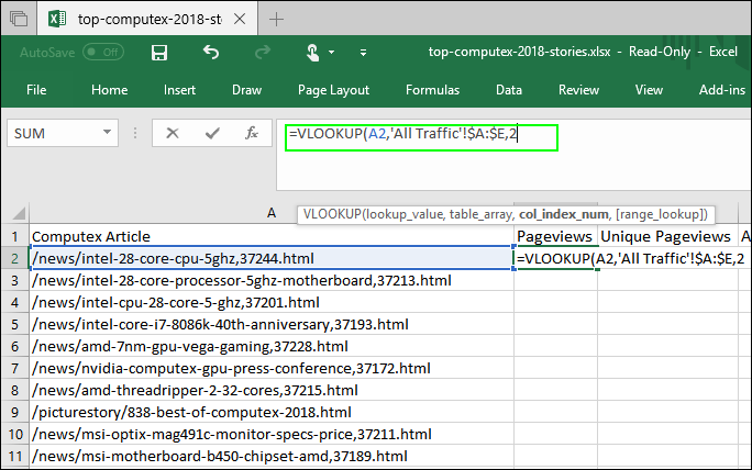
5. Highlight the cell range in the formula and hit F4. The application will put dollar signs on the cell range to signify that these are absolute addresses, which means that you won't need to redo this part of the formula if you paste it into another cell.
6. After inserting a comma, enter the column number of the data you want to copy over to the primary sheet. In our case, the Page Views column we want to copy is second from the left (column B), so it is number 2. Note that the column number you need is the one from the data sheet, not the primary sheet.
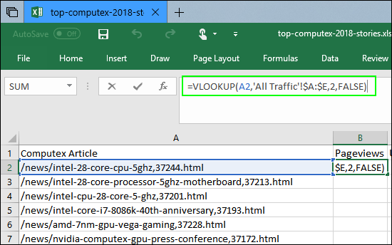
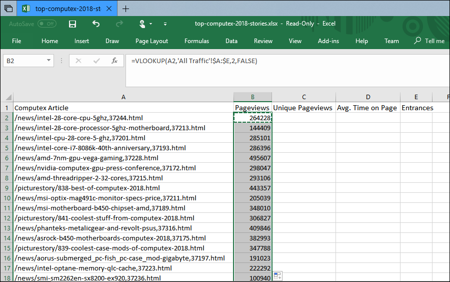
7. Enter comma followed by the word FALSE and then a close parenthesis. Entering FALSE ensures that VLOOKUP accepts only an exact match. That's your complete formula.
8. Copy and paste the formula down the entire column.
If you want to import other columns, copy the formula over to a cell in another column, but be sure to change the destination cell (in our case, from 2 to 3 or 4) and keep the matching cell at what it was (A2 in our case).
Avram Piltch is Managing Editor: Special Projects. When he's not playing with the latest gadgets at work or putting on VR helmets at trade shows, you'll find him rooting his phone, taking apart his PC, or coding plugins. With his technical knowledge and passion for testing, Avram developed many real-world benchmarks, including our laptop battery test.
-
elroy.coltof Please don't, I swear a kitten is killed everytime someone uses VLOOKUP when INDEX should be used. I've spent too many wasted hours fixing painfully slow excel sheets that do searches when a direct indexing is possible.Reply
The kitten is only maimed if you use VLOOKUP when INDEX and MATCH should be used. INDEX and MATCH are much more robust against column insertions and you can directly read what column your results will be pulled from. Not to mention the huge advantage that you can now skip repeating your key column because you couldn't count out the 20+ columns in between to determine the column number in your vlookup search area. (The key column could even be to the right of your results column, but try to prevent that if at all possible. -
anbello262 Useful article! I use Excel all the time and only learnt about this function recently, so keep these coming!Reply -
Soaptrail As an accountant we hired a senior accountant who did not know how to do a vlookup. I was flabergasted. But i knew he would not last long at our company and I was right. Excel is everyone's best friend they just don't realize it.Reply -
silverblue Ah VLOOKUP... how I dislike you. Articles on INDEX and MATCH would be very helpful, especially when somebody's working with a lot of data (and especially when you're on a fair to middling laptop).Reply
Array formulas take the cake, though. :) -
derekullo I need better Excel skills like / unlike this; not sure judging by comments.Reply
At work I do alot of traveling between locations pretty much at random.
I may go from branch 4 to branch 2 on Monday and then branch 7 to branch 1 to branch 11 on Tuesday.
So in an effort to make it easier to calculate distances between branches I hard coded in excel's visual basic "i believe it's visual basic" the distance between all 16 branches to every other branch on the spreadsheet for the first 3 lines on the excel page.
if a1 = branch 1 and a2 = branch 2 then a3 = 4 (distance between branches)
Each row in excel has at minimum 16x16 or 256 if then statements
So with 3 rows I choose to write that's 256x3 or 768 lines of code instead of a chart lookup table thingy.
Payroll also wants the actual name of the branch so I made another hard coded script that replaces "branch 1" with the actual name and address of the branch.
If a1 = branch 1 then a1 = Branch 1 Street, Streetville, OH
This effectively doubles the previous number from 768 to 1536 lines of code.
I am 99% sure this is the wrong way to do it but this 1500+ line monstrosity works well and is remarkably quick. -
hermitboy A little history could be nice as well - which can help with optimization.Reply
Back when computers were much less powerful, doing any sort of lookup could take a really long time.
Then along comes Vlookup.
Vlookup works best when your data is sorted, because it was created with a specific shortcut in mind - narrowing the search range by half.
Vlookup compares your lookup value to the middle value in the primary column. Then it will compare the lookup value to middle of the top half or bottom half - and will continue comparing the lookup value to increasingly smaller ranges until it finds the match.
Not sorting the data defeats the purpose of Vlookup's shortcut processing - and can make the actual lookup take much longer than if Index-Match were used.
Personally, I prefer index-match. Especially in situations where I need the data sorted on a column that is not related to the lookup value. But there are times when I'll use Vlookup instead. -
elroy.coltof Reading back all the comments I feel it's best to explain why VLOOKUP is a terrible choice for this particular problem.Reply
First off it should be noted that VLOOKUP has two wildly different modes of operation. If the last parameter is TRUE (the default if you omit it) it expects a sorted first column and is really fast using a binary search. However it also means it looks for an aproximate match. If the value you look for is not in the table it returns the closest result after the position after where your result should have been. BUT IT DOESNT TELL YOU THIS! The search is O(logN)
The second mode, last parameter FALSE looks for an exact match and does not require sorted data, it does a lineair search and is bog slow. It does however return an N/A if no exact match is found. The search is O(N).
To speed things up therefore you could sort the data you're searching in and use a double aproximate vlookup in an if statement: The first one you is in the condition and checks against the search value, if they are different then the item is not present, return N/A manually. If they are equal do the VLOOKUP again and return the value. If you do it in this order at least the second lookup would not be done if an item is not present. If you have a large amount of data and you are able to sort them this is faster than a single exact vlookup! Never use FALSE on large sorted datasets!!
Now consider that if you want to merge multiple columns you have to repeat those VLOOKUPs for every column, so 20 columns is 20x as slow!
And now INDEX/MATCH: The power here is that they are two different functions.
INDEX allows you to take a range and directly reference a value in that range by row and column number. No searching happens, it's O(1)!
MATCH determines the row number the matching item is in using a lineair search (the slow one, I know, but because of the way it's implemented it's still faster and uses less memory). You can store this value in a cell and then use Index for every column you want to match. It's O(N) for an exact match (last param = 0) and O(log(N)) for an aproximate search (last param = -1 or 1) and you only have to do it once for every row and not for every column! You can do the same trick with a double aproximate MATCH as you could do with VLOOKUP to benefit from the speed of binary search and still be guarantueed to be told if there is no exact match.
So how do you then match up to data tables with the same key column?
You make a helper column with MATCH that has the row numbers in the second file in the order they appear in the first file. This column can be on a different sheet or even in a different file. And then you use INDEX to add the data to the first file. -
punakuca48 Everything that Elroy said about VLOOKUP (not to mention notorious LOOKUP) is right. Today. But, VLOOKUP was made in times when spreadsheet was ment to be spreadsheet, and not database as is case today. Times when you were very limited by size of the spreadsheet and where people would be making small tables (coutning hundreds of rows) where VLOOKUP made sense. It still does if your tables are small and you want fast rezults.Reply
I use it on dayly basis in such cases, but if tables grow over 10000 rows INDEX/MATCH combo cannot be beaten! Especially if you have 50+ columns and key column is third or 10th and not the first one.
Also purpose of TRUE variant and FALSE variant are totaly different! TRUE variant gives you exact match when that match exists. But if you deal with ranges and only limits of the ranges are quoted in compare to table, FALSE variant is the only one usefull and right. -
peter.domanico I’ve taken this to the next level here: (Excel only):Reply
https://codereview.stackexchange.com/q/196125/138859
Enjoy!
