When you're working with spreadsheets, sometimes you need to match up data from two different worksheets that have one cell in common. Perhaps you have a list of employee names with their ID numbers and another list with names and addresses or maybe it's a list of web articles with traffic data on one sheet and author names on another. That's where Excel's new XLOOKUP function comes in.
First added to current release versions of Excel in February 2020, XLOOKUP is meant to improve upon the popular VLOOKUP function, which also combines data from different sheets, but has less functionality. It also does everything that HLOOKUP, which finds data in the same column as the data you searched for.
Advantages of XLOOKUP over VLOOKUP
- Can copy multiple columns at once.
- Doesn't require the reference cell to be in first cell on the left
- Defaults to exact matches only (VLOOKUP didn't)
- Can use wildcards for inexact matches
- Lets you specify "not found" text for when there are no matches
- Only three required parameters
XLOOKUP accepts up to six parameters, but only the first three are required. It's formatted as:
Article continues below=XLOOKUP(lookup_value,lookup_array,return_array,[if not found],[match_mode],[search_mode])
Let's start by showing how to do a simple XLOOKUP query.
How to Do a Simple XLOOKUP Query
1. Type =XLOOKUP( into the first cell where you want the results to appear.

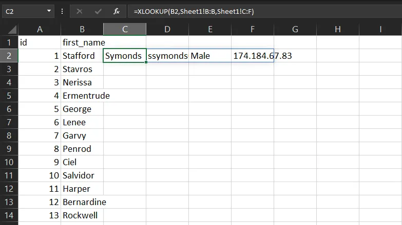
2. Click the cell which contains the lookup_value and enter a comma (you can also type the cell address -- ex: C2). That's the value you're checking against in both sheets. In our example, the lookup_value is cell C2, which contains the last name. You could also just write the value in quotes, but then you couldn't copy and paste it down a series of rows and get different matches for each.

3. Select the range of cells to search for the lookup_value and add a comma. We strongly recommend that you select a full column, rather than just highlighting the cells with data in them. That way if you copy and paste, the range will say the same.
Again, you could type in the range manually but highlighting with your mouse is probably easiest. This column can be in a different tab of the same Excel file or even in a completely different file on your computer. In our case, we're choosing all of column B on the Addresses tab of our file, because it also contains the last name.

4. Select the range of cells to return and then add a close parens to complete the function call. Again, we recommend selecting full columns. If you choose more than one column's worth of data, all of the columns after the fist one will be copied into cells that are adjacent to your XLOOKUP formula.
In our case, we selected columns C through E in the Addresses sheet so we could carry over the email addresses, gender and IP addresses of the employees. Our final formula looks like:
=XLOOKUP(C2,Addresses!B2:B1001,Addresses!C2:E1001)

You'll get an end result that looks like what you see in the image below.

5. Copy and paste the formula into other cells to use it across an entire set of rows. If you drag the formula down to the last row with data, Excel will automatically replace the lookup value cell with the appropriate row number. So, if your first cell was C2 and you copy the formula into row 500, it will be C500.

However, if you didn't select a full column for your lookup_array or return_array parameters, you'll need to add $ signs to the cell ranges before you copy and paste. Otherwise, the range of cells you're searching will change as you paste into lower rows. The fastest way to add dollar signs is to highlight those portions of the formula and hit the F4 key.

XLOOKUP's "If Not Found" Parameter
If you don't fill in a fourth parameter in XLOOKUP, any failed searches will show up as #N/A. But if you want to customize the message (or leave it blank) for cells , just add a not-found message in quotes.
In our case, we used the text "Sorry, did not find this." Our formula now looks like:
=XLOOKUP(C2,Addresses!B2:B1001,Addresses!C2:E1001,"Sorry, did not find this.")

XLOOKUP's Match Mode
By default, XLOOKUP only returns exact matches so, if it's searching for the last Symmonds and, on another sheet, it's spelled Simmonds, there's no match. Or, if you're searching for a numeric value like "300," and there are higher or lower numbers, you won't get a match.
However, for the fifth parameter, you can select a "match mode" which has Excel search for a wildcard, the next largest or the next smallest number. Mode 0, the default, is an exact match. Entering -1 will look for the next smallest item if an exact match isn't found. So if it's looking for 300 and there's a 200 and a 400 instead, it will return the 200. Match mode 1 gives you the next largest number (the 400).

Match mode 2 lets you use wildcard characters to search. The wildcard * will match any number of characters while the ? character is used for just one. So, if you want to find either "Symmonds" or "Simmonds," use "S?mmonds" in match mode 2. If you want to find the first name that begins with S, you can use "S*" in match mode 2.
XLOOKUP Search Mode
The sixth and arguably least important XLOOKUP parameter controls the way that Excel searches. For most people and situations, we'd skip this parameter entirely, because it probably won't change much.

For search mode, you have four options. Mode 1, the default, begins searching at the top row in your search range and finds the first match. Mode -1 searches from the bottom up. Mode 2 (first to last) and -2 are for binary searches. For binary, you need to have the data sorted and the system compares each cell to the middle value in the column and, if it doesn't match, it contracts the search further. Honestly, I don't know why you'd need this, but it might be faster on huge data sets.
